
Application Note
Parallel line analysis and relative potency in SoftMax Pro GxP and Standard Software
- Apply a constrained global fit with the click of a button
- View automatically-calculated relative potency, curve fit parameter, and confidence interval values
- Test for parallelism using pre-written parallel line analysis protocols
- Perform parallel line analysis and calculate relative potency using software features that support FDA 21 CFR Part 11 and EudraLex Annex 11 data integrity regulations
Introduction
In laboratories operating under GMP (good manufacturing practice) and GLP (good laboratory practice) regulations, biological assays are frequently analyzed with the help of parallel line analysis (PLA). PLA is commonly used to compare dose-response curves where there is no direct measurement of a product, but rather an effect is measured (Figure 1). Parallelism methods allow the user to establish if the biological response to two substances is similar or if two biological environments give similar dose-response curves to the same substances. Testing for parallelism is a prerequisite to calculate the relative potency of a compound and plays an important role in many pharmaceutical drug development applications such as drug comparison, analyte confirmation, crossreactivity, interfering substances, matrix compensation, concentration estimation, and inhibitory studies.

Figure 1. Parallel line analysis of dose response data sets with a constrained global 4-parameter curve fit.
Two curves are defined to be parallel when one function is obtained from the other by a scaling factor either to the right or to the left on the x-axis, ƒ(x) = ƒ(rx), where x is the dose and r is the scaling factor, or relative potency.1 The relative potency is generally set to one for the reference curve (known agent) and the scaling factor used to transform the reference curve into the test curve (unknown agent) is the relative potency of the unknown agent. This methodology works well for linear regression curve fits where the slope is unchanged across the concentration range (Figure 2). However with non-linear regression curve fits, such as the 4-parameter and 5-parameter logistics, the sigmoidal dose-response curve has a variable slope over the entire concentration range (Figure 1).

Figure 2. Parallel line model for linear regression. The relative potency is set to one for the reference curve (red circle) and the scaling factor used to transform the reference curve into the test curve (blue diamond) is the relative potency of the unknown agent.
Methods testing parallelism can be divided into two categories depending on how the parallelism hypothesis is tested: response comparison tests and parameter comparison tests.1 This application note explains both methods and outlines how to use them in SoftMax® Pro GxP and Standard Software to test for parallelism. A protocol has been implemented with the F-test probability using the F-test1,2 and the chi-squared probability with the chi-squared test3. Furthermore, a parameter comparison method has also been developed using Fieller’s theorem. This protocol is called Parallelism Test and is located in the SoftMax Pro Protocol Library in the Data Analysis subfolder. All of these methods can be used for linear and non-linear regression curves.
Testing for parallelism
Response comparison test
Biological systems often do not behave as expected and generally add noise and variation to the data. Therefore, choosing the correct curve fit model and applying a weighting factor, if necessary, that can accommodate these variations is the first important step to consider before parallelism analysis. If an inappropriate curve fit model is selected, it could introduce bias into the parallelism metrics and may lead you to the wrong conclusion.
Calculating the relative potency of non-parallel curves is difficult due to the rare occurrence of curve fits that are perfectly parallel for assay data, especially for non-linear regressions. With the response comparison method, the tested curves are simultaneously fit into a constrained model, where the curves are forced to be parallel, and an independent model, where the curves are independently fitted. Statistical metrics are then used to compare differences in the goodness of fit between the constrained model and the independent model, which might be attributed to non-parallelism.
When fit to the constrained model, parameters describing the curves are identical for all curves except for the parameter describing the X-value. For a linear curve, the X-value is the intercept and for a non-linear curve, the X-value is the midpoint between the upper and the lower asymptotes, which is the EC50. SoftMax Pro Software includes tools to determine the relative potency of linear fits as well as evaluate non-linear curves using both the constrained or global fit model and the independent model for relative potency estimation.
Testing the null hypothesis
With the response comparison method, the calculated parallelism metrics are often a function of the residualsum of squared-errors (RSSE) and determine how well the constrained model fits the data. One specific method has been developed and uses the Extra-Sum-of-Square analysis1,2. This statistical regression technique is a form of analysis of variance (ANOVA) where the null hypothesis is that the constrained model is correct, or that the curves are parallel. The null hypothesis can be tested using various statistical techniques including the F-test probability with the F-test1,2 or the chi-squared probability with the chi-squared test3. For both methods, the probability is reported as a number between zero and one. As the probability becomes closer to one, it is more likely that the curves are parallel. It is important to note the deficiencies of the F-test. The F-test can result in a false positive for well-fitting independent curves or a false negative for independent curves with a poor fitting. These two statistical methods have also been included in SoftMax Pro Software. Values of the test and the probabilities can be obtained easily with the following formulas:
- ChiSquaredPLA (PlotName@GraphName): Returns the value of the chi-squared statistic for a reduced curve fit.
- ChiProbabilityPLA (PlotName@GraphSection): Returns the chi-squared probability distribution value for a reduced curve fit.
- FStatPLA(PlotName@GraphSection): Returns the value of the F-test statistic for a reduced curve fit.
- FProbPLA(PlotName@GraphSection): Returns the value of the F-test probability for a reduced curve fit.
Note: All of the above formulas can be used only when the Global Fit (PLA) option is enabled in the Curve Fit Settings dialog. PlotName@GraphName is the full name of the plot, including the name of the graph. For example, Plot#1@Graph#1 or Std@Standardcurve. The designation of a specific plot is arbitrary since the chi-squared value is calculated from all plots in the designated graph.
A protocol titled “Parallel Line Analysis Using F-test and Chi-squared Test” has been developed to test for parallelism according to these two statistical testing methods. Once the data is acquired or imported into the protocol, the calculations will occur automatically and assess whether or not the null hypothesis, that the curves can be considered parallel, is true.
In this protocol, the probability results for the F-test and the chi-squared test must be above 0.05 for the curves to be considered parallel. Roughly speaking, with this setting, there is 95% confidence that the null hypothesis is true. The confidence level can be adjusted as needed to an acceptable level of non-parallelism for the assay performed.
Noise and weighting
Noise is defined as the random variability of measured response. It is an important factor to consider when parallelism is assessed as it affects the ability to detect non-parallelism. At a high noise level, parallelism metrics can no longer measure non-parallelism as it is less than the amount of noise.
The F-test and the chi-squared metrics handle the expected noise levels differently in the calculation of their probability. While the F-test probability is unaffected by this factor, the chi-squared probability is highly dependent on noise levels and requires that data variances are correctly estimated. It is therefore necessary to have inverse variance weighting when the chi-squared method is used.
As discussed in the application note “Selecting the best weighting factor in SoftMax Pro GxP and Standard Software”, bioassays tend to have a much larger variance in the upper part of the curve. With unweighted regression, the parallelism results can be dominated by the data points from the top of the curve, and information from the lower part of the response curve does not contribute much.
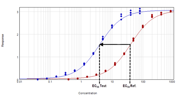
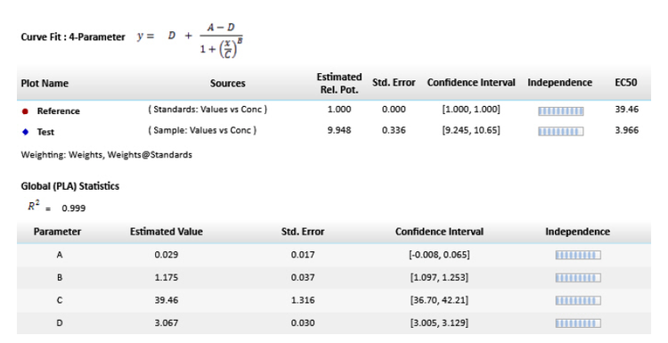
Figure 3. Parallel line model for non-linear regression. The relative potency is determined in the linear region of the curve where the response changes relative to the concentration at 50% effective dose or EC50. The curves tested are fitted to the constrained model. The parameters describing the curves are identical for all curves except for the X-value in the 4-parameter curve fit equation.
In the software protocol, the weighting factor used is the inverse of the variance, but this can be adjusted to a more suitable weighting factor if needed. In addition, there is an option to specify that the weights are to be treated as inverse variances (Figure 4G). The chi-squared profile method for parameter confidence intervals (Figure 4H) is only available when the ‘Weights are Inverse Variances’ box is checked. An optimal weighting factor will ensure that the results are not dominated by the most variable data points.
How to apply PLA in SoftMax Pro GxP Software
In the software, PLA is available for all global curve fits except point-to-point, log-logit, and cubic spline. In a graph section, all the plots will have the same curve fit functions applied. PLA can be implemented as shown in Figure 4.
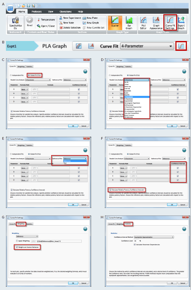
Figure 4. How to apply PLA in SoftMax Pro GxP and Standard Software and estimate relative potency. Select a graph section with multiple plots. Click Curve Fit in the Graph Tools section on the Home tab in the ribbon (A) or in the toolbar at the top of the graph section (B). (C) In the Curve Fit Settings dialog, select Global Fit (PLA). (D) Select any curve fit option except point-to-point, log-logit, or cubic spline from the drop down list. (E) Select a plot for the Reference Plot list. (F) If applicable, select the curve fit parameters and the Relative Potency Confidence Intervals. (G) If applicable, click the Weighting tab. See Application note “Selecting the best weighting factor in SoftMax Pro GxP and Standard Software”. You may also directly select the inverse of the variance weighting factor. (H) If applicable, click the Statistics tab. (I) When all curve fit options have been selected, click OK. The curves tested are fitted to the constrained model. The parameters describing the curves are identical for all curves except for the parameter describing the X-value as shown in Figure 3. For non-linear functions, the minimum and maximum responses (lower and upper asymptote, respectively) are also constrained to be the same for all curves.
Parameter comparison method
Unlike the response comparison methods that directly assess differences in the dose-response curve, the parameter comparison methods individually compare the parameters of unconstrained curves to an approximate confidence region. The parameter pairs must fit within this defined confidence interval according to a specified level of confidence. This type of evaluation is called equivalence testing and tests for a degree of parallelism less than a specified threshold. The slope ratio method used by the European Pharmacopoeia is one example of equivalence testing.
Fieller’s theorem
Fieller’s theorem uses statistics to calculate the confidence interval for the ratio of two parameters.4 The tInv function is used to calculate the estimated ratio and therefore follows a Student’s t distribution with degrees of freedom for which the probability is p. Statistical formulas in SoftMax Pro Software allow you to calculate the confidence interval for the ratio of a curve fit parameter between two curves such as reference and test curves. A protocol (Figure 5) has been developed incorporating these calculations with a probability set to 0.1 (90% confidence), which may be adjusted as needed. In order to determine whether the reference and the test curves are considered parallel, the calculated confidence interval is compared to a fixed confidence interval defined by a certain confidence level. In the protocol, a 90% confidence level is applied; therefore the calculated confidence interval should be within 0.9 and 1.1 for the curve to be considered parallel.
For linear regression curves, this test is applied to the slope values of the reference and the test curves, which are described by the B parameters in SoftMax Pro Software. However for non-linear regression curves, parameters describing the upper asymptote and the slope are tested. The lower asymptote is not tested as this is a mathematical limitation of the Fieller’s theorem. At a lower concentration, the variance of the parameter is too high and generates an intermediate calculation containing imaginary numbers which result in a final calculated confidence interval that is either incorrect or cannot be calculated. This issue has been addressed by the United States Department of Agriculture (USDA) Center for Veterinary Biologics with a recommendation to fix the lower asymptote to zero and use the slope and the upper asymptote for the tests5. Similarly, the Parallelism Test protocol included in SoftMax Pro Software automatically sets the lower asymptote to zero and tests the slope (Parameter B) with either Parameter A or Parameter D as the upper asymptote to determine if the reference and the test curves can be considered parallel (Figure 5).

Figure 5. Response comparison method in SoftMax Pro Software to assess parallelism. The confidence level and the probability are set to 90 % and 0.1 respectively, but can be adjusted as needed. Once the lower (rBCILower and rDCILower) and upper (rBCIUpper and rDCIUpper) values of the confidence interval for the parameter ratio have been calculated, they are compared to a defined confidence interval (lval and uval). If the calculated confidence interval values are within that defined confidence interval, then the reference and the test curves can be considered parallel for that parameter.
Conclusion
Many biological assays require parallelism determination between pairs of dose-response curves. This application note describes response comparison methods, such as the F-test and chi-squared test, and parameter comparison methods, illustrated with Fieller’s theorem. SoftMax Pro Software enables you to choose between a constrained or an unconstrained curve fit model and provides advanced statistical formulas for analysis. The software also includes a pre-written protocol developed with different sections for each test so you may choose the appropriate method to easily evaluate parallelism for some or all of the parameters describing two curves.
Together with SoftMax Pro GxP Software’s data integrity features, assessing parallelism and calculating relative potency can be performed in FDA 21 CFR Part 11 and EudraLex Annex 11 compliant laboratories.
References
- Gottschalk, P.D. and Dunn, J.R. 2005. Measuring parallelism, linearity, and relative potency in bioassay and immunoassay data. Journal of Biopharmaceutical Statistics 15(3): 437-463.
- Bates D. M. and Watts D. G. 1988. NonLinear Regression Analysis and its Applications. New York, Wiley.
- Draper, N. R. and Smith H. 1998. Applied Regression Analysis. 3rd Ed. New York, Wiley.
- Buonaccorsi, J. P. 2005. Fieller’s Theorem. In: Armitage, P., Colton, T., editors. Encyclopedia of Biostatistics. 2. Vol. 3. New York, Wiley.
- United States Department of Agriculture Center for Veterinary Biologics Standard Operating Policy/Procedure. 2015. Using Software to Estimate Relative Potency. USDA Publication No. CVBSOP0102.03. Ames, IA.